Seng Kwang Tan

Safety Features in a Household Circuit

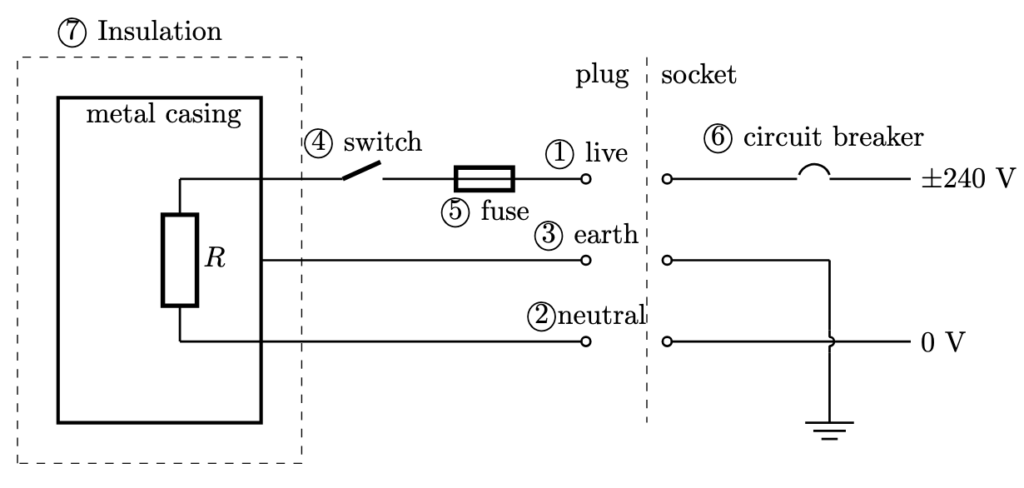
  1. Live wire: wire carrying the current at a high voltage from the power source to the electrical appliance.
  2. Neutral wire: wire completing the circuit by carrying current back to the power source, maintaining a low potential close to zero volts.
  3. Earth wire: wire provides a path for electrical current to flow safely into the ground in case of a fault, preventing the appliance’s exterior from becoming live and reducing the risk of electric shock.
  4. Switch: a device that opens and closes the circuit. Connected to the live wire instead of neutral wire so that device does not remain live when current is off.
  5. Fuse: a safety device connected to the live wire and is designed to melt/break, thus creating an open circuit, when the current passing through it exceeds a specified value. Its current rating should just be slightly higher than the normal operating current.
  6. Circuit breaker: a safety device connected to the live wire which switches off the electrical supply when a excessive current flows through it.
  7. Double insulation: two layers of protection to prevent users from coming into contact with live electrical parts, eliminating the need for an earth connection.

Example Scenarios

Fault: You accidentally run over the iron’s cord with a chair, exposing the internal wires. Exposed live wire touches the metal casing.

Protection:

  • Earth Wire diverts the fault current safely to the ground.
  • Circuit Breaker detects the sudden surge and cuts off power immediately OR
  • Fuse in the plug blows to break the circuit.
  • If the appliance had Double Insulation, the user will not be able to touch the metal casing.

Fault: You plug too many devices into the same extension cord, leading to overloading — the total current drawn exceeds the safe current rating.

Protection:

  • Fuse in the plug blows to break the circuit.
  • Circuit Breaker in the consumer unit (distribution board) trips, cutting off power.

Simulation of Projectile Motion with Air Resistance

Open in new tab 🔗 This simulation offers a hands-on and dynamic way to explore the physics of projectile motion with and without air resistance. By adjusting parameters such as launch velocity, angle, and air resistance, users can visualize how these factors affect the shape and reach of a projectile’s trajectory. The app provides real-time changes including motion paths, velocity vectors, and a velocity-time graph showing horizontal and vertical components separately. It also calculates and displays key quantities such as maximum height and range under ideal and non-ideal conditions (based on an arbitrary coefficient of drag. Through interactive experimentation and visual reinforcement, learners gain a deeper understanding of concepts the effect of air resistance, and the difference between theoretical and real-world motion. This is suitable for JC1’s topic on projectile motion. It can also be used for Upper Sec, if you change the launch angle to 90 degrees.

Interactive System Schema Generator

I built this web app to help students draw system schemas, having blogged about this before.

It is also available and optimised for download for SLS.

Basic Instructions

To add Bodies:

  • Click the “Add Body” button.​
  • Click on the canvas to place the body at your desired location.​
  • Label the Body.

Add Forces:

  • Click the “Add Force” button.​
  • Click on two bodies that exert the force on each other.​
  • Label the Force.

Using System Schema to Understand Newton’s Third Law

Newton’s Third Law states that when Body A exerts a force on Body B, Body B exerts an equal and opposite force on Body A. While this principle is conceptually simple, many students struggle to apply it consistently across different physical scenarios. The System Schema approach provides a powerful way to visualise and analyse these interactions. It is a representation tool developed by The Modeling Instruction program at Arizona State University (Hinrichs, 2004).

A system schema is a diagram that represents objects (as circles) and interactions (as lines) between them. Instead of focusing on individual forces, a system schema helps students see the relationships between objects before applying force diagrams. This method emphasizes Newton’s Third Law by explicitly showing how forces come in pairs between interacting objects.

To correctly identify action-reaction force pairs, consider the following guidelines:​

  1. Forces Act on Different Objects: Each force in the pair acts on a different object. For example, if Body A exerts a force on Body B, then Body B simultaneously exerts an equal and opposite force on Body A.​
  2. Forces Are Equal in Magnitude and Opposite in Direction: The magnitudes of the two forces are identical, but their directions are opposite.​
  3. Forces Are of the Same Type: Both forces in the pair are of the same nature, such as gravitational, electromagnetic, or contact forces.

The steps to applying System Schema to Newton’s Third Law are as follow:

  1. Identify the bodies in the system – Draw each object as a separate circle.
  2. Represent interactions – Draw lines between bodies to indicate forces they exert on each other (e.g., a box on the ground interacts with Earth through gravitational force).
  3. Label force pairs – Each interaction represents an action-reaction force pair (e.g., a hand pushes a wall; the wall pushes back).
  4. By mapping forces this way, students can easily recognize that forces always act between bodies and in pairs, reinforcing the symmetry of Newton’s Third Law.

One of the most common misconceptions of students is that normal contact force and gravitational force acting on a body are action-reaction pairs because they are equal and opposite in a non-accelerating system. By using the system schema, they can see that the two forces involve interaction with different bodies, e.g. the floor of an elevator for normal contact force, and the Earth for gravitational force.

Kinematics Graphs Interactive

Understanding motion in physics often involves analyzing displacement, velocity, and acceleration graphs. With the interactive GeoGebra graph at this link, you can dynamically explore how these concepts are connected.

How It Works

This interactive simulation lets you visualize an object’s motion and its corresponding displacement-time, velocity-time, and acceleration-time graphs. You can interact with the model in two key ways:

  1. Adjust Initial Conditions:
    • Move the dots on the graph to change the starting displacement, velocity, or acceleration.
    • Observe how these changes influence the overall motion of the object.
  2. Use the Slider to Animate Motion:
    • Slide through time to see how the object moves along its path.
    • Watch the displacement vector, velocity vector, and acceleration vector update in real time.

Key Observations

  • When displacement changes, the velocity and acceleration graphs adjust accordingly.
  • A constant acceleration results in a straight-line velocity graph and a quadratic displacement graph.
  • Negative acceleration (deceleration) slows the object down and can cause direction reversals.
  • If velocity is constant, the displacement graph is linear, and acceleration remains at zero.

Why This is Useful

This GeoGebra tool is perfect for students and educators looking to build intuition about kinematics. Instead of just solving equations, you get a visual and hands-on way to see the relationships between these key motion variables.

Try it out yourself and experiment with different conditions to deepen your understanding of motion!

Exploring Motion with a Ticker Tape Timer

This week, I conducted a lesson on motion for my IP3 class using a simple yet effective tool: a simulated ticker tape timer. The objective was to help students develop an intuitive understanding of uniform and non-uniform motion by actively engaging in an experiment.

Introduction to the Ticker Tape Timer

To kickstart the lesson, I showed my students a YouTube video that explains how a ticker tape timer works:

This video provided a visual demonstration of how a ticker tape timer marks regular intervals on a moving strip of paper, allowing us to analyze motion quantitatively.

Hands-On Experiment: Simulating a Ticker Tape Timer

After the video, I had students pair up for a hands-on activity. Instead of using an actual ticker tape timer, we simulated the process using paper strips cut from A3-sized sheets. Each pair had one student act as the “moving arm,” responsible for placing dots on the strip, while the other played the role of the “puller,” responsible for pulling the paper strip at different speeds.

To ensure a consistent time interval between each dot, I used a Metronome App that I created:

This app produces a steady rhythm at 120 beats per minute, meaning that the interval between each beep (and consequently each dot) is 0.5 seconds. To improve accuracy, the student acting as the moving arm was instructed to close their eyes and focus solely on the beep.

Step 1: Recording Uniform Motion

In the first trial, the puller was asked to pull the paper at a constant rate. As the paper moved steadily, the moving arm marked dots at regular intervals based on the metronome beat. After completing the trial, students used a ruler to measure the distances between successive dots. Since the time interval was fixed, they could easily calculate the speed of the paper by using:

Step 2: Recording Accelerated Motion

Next, the students switched roles. This time, the new puller was asked to gradually increase the speed of the paper. As expected, the spacing between dots increased progressively, providing a clear visual representation of acceleration. This led to discussions on how motion can be analyzed using dot patterns and how acceleration differs from uniform motion.

Reflections and Key Takeaways

This activity was highly effective in reinforcing key motion concepts. Since we do not have an actual ticker tape machine, it allowed students to engage in a hands-on simulation while visually and physically experience motion rather than just reading about it.

Next Steps

To extend this lesson, I plan to introduce velocity-time graphs and have students plot their measured speeds to analyze changes in motion further. Additionally, incorporating digital tools like video analysis with Tracker software could help reinforce these concepts further.

If you have any feedback or suggestions, feel free to share them in the comments below!

Symposium on Tech for Engagement at SISTC 2024

This deck of slides are the ones I will be using for the Symposium on “Leveraging Technology for Engaging and Effective Learning” at the Singapore International Science Teachers’ Conference (SISTC) 2024 on Day 2 of the Conference (20 November). Feel free to download for your reference.