I bought a simple beta Stirling engine online at dx.com recently and it came in the mail today. It works well with a cup of hot water placed under it, although it might take a little push to get it started due to the initial static friction. However, once it starts spinning, the wheel goes on and on for a very long time.
From the video, you can observe the expansion of the air within the main piston cylinder as the heat below raises the temperature and pressure. This forms the power stroke. When the piston rises, it pushes air into a secondary piston, which also helps to provide torque to the wheel. When the air in both pistons expand, it cools down. An understanding of the 1st law of Thermodynamics (JC syllabus) is necessary to appreciate why that happens. Upon cooling, pressure decreases and the pistons fall. The cycle repeats itself.
This is the Pendulum Clock from the LEGO Education Simple and Powered Machines Set. It can be used to demonstrate the variation of period with length of pendulum and is a very good visual representation of the escapement mechanism.
There are many other models that one can build using this set, including a weighing scale, elastic energy powered car, etc. All with potential for class demonstrations.
You can buy a set from Duck Learning in Singapore at (S$329.75), an exclusive distributor of LEGO Education products in Singapore. If you are purchasing in bulk for your school, you may want to contact them directly for a package deal. You can also purchase them from overseas sites such as Bricklink.com if you can find them at a better price.
For my students: To download the file and video for analysis using Tracker, right-click the file here…
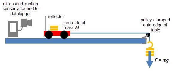
To verify the equation F = ma, where F is the resultant force on an object, m is the mass of the object and a is the acceleration, this is one of the ways to do so:
Equipment:
1. Motion Sensor
2. Datalogger
3. Cart with variable mass
4. End Stop
5. Pulley with clamp
6. Hanger Mass Set
7. String (about 1.2 m)
For a system of a cart of mass M on a horizontal track that is connected to a hanging mass m with a string over a pulley, the net force F on the entire system (cart and hanging mass) is the weight of hanging mass. F = mg (no friction assumed).
According to Newton’s Second Law, mg = (M+ m)a. We will try to prove experimentally that this is true in the video below.
The following is a question (of a more challenging nature) posed to JC1 students when they are studying the topic of kinematics.
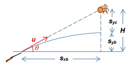
A gun is aimed in such a way that the initial direction of the velocity of its bullet lies along a straight line that points toward a coconut on a tree. When the gun is fired, a monkey in the tree drops the coconut simultaneously. Neglecting air resistance, will the bullet hit the coconut?
Two-Dimensional Kinematics: Gun and Coconut Problem
It is probably safe to say that if the bullet hits the coconut, the sum of the downward displacement of coconut and the upward displacement of the bullet must be equal to the initial vertical separation between them, i.e.
This is what we need to prove.
Since
and
At the same time, the relationship between and the horizontal displacement of the bullet before it reaches the same horizontal position of the coconut is
I’ve used the open-source Tracker software, a video analysis and modeling tool built for use in Physics education, for both my IP3 and JC1 classes this year. Thanks to Mr Wee Loo Kang and his team for enthusiastically introducing this software to the physics teachers of Singapore.
For the IP3 cohort, students were tasked to analyse the movement of any sports-related projectile and to relate the variations in displacement, velocity and acceleration to one another in both dimensions. This was a direct transfer task for the topic of two-dimensional kinematics that they were taught in class. Attempts to explain these variations using the idea of forces were encouraged as well, even though that topic has not be formally introduced yet.
For my JC1 class, I explained the specific example of the bouncing ball using the software, which was useful to show the variation in vertical displacement, velocity and acceleration synchronously with the positions of the ball. I used the resources in the Singapore Tracker Digital Library, search for the following directories: 02_newtonianmechanics_2kinematics > trz > Balldropbounce4x.trk.
Use of Tracker to explain the bouncing ball graphs
It was easier for students to compare the three stages of the movement, namely Stage A: the way up, Stage B: the bounce (during which the ball is in contact with the ground) Stage C: and the way down.
A series of guiding questions such as the following will be useful:
Is there a difference between the vertical accelerations in stages A and C?
What do the gradients in the velocity time graph for stages A, B and C represent?
Identify the turning point of the ball in all 3 graphs. Notice that the acceleration remains at about 10 m s-2.
How would the graphs look like if the coordinate system / sign convention is changed such that the displacement is defined as zero at the floor and upward is taken to be positive? The effect of this change can be shown by dragging the axes on the video (the two perpendicular purple lines) to the bottom and rotating the horizontal axis 180o; by dragging the short purple line near the intersection.
Graphs with different coordinate system defined.
The following video (sorry, no audio) shows the steps to take to do all the above. Just pause it at any point and rewind if you didn’t catch what I did.