29 January
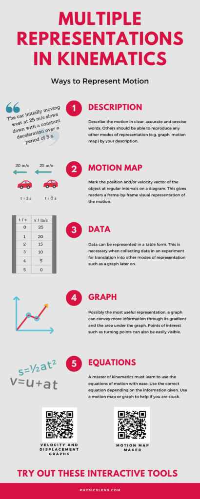
This is another Infographic made using Canva last year.
the world in a different light
This is another Infographic made using Canva last year.
Through this GeoGebra app, students can observe how the gradient of the displacement-time graph gives the instantaneous velocity and how the area under the velocity-time graph gives the change in displacement.
In the GeoGebra app below, you will see a displacement-time graph on the left and its corresponding velocity-time graph on the right. These graphs will be referring to the same motion occuring in a straight line. Instructions
This GeoGebra app allows students to observe the difference between instantaneous and average velocity from a graphical perspective.
I’ve used the open-source Tracker software, a video analysis and modeling tool built for use in Physics education, for both my IP3 and JC1 classes this year. Thanks to Mr Wee Loo Kang and his team for enthusiastically introducing this software to the physics teachers of Singapore.
For the IP3 cohort, students were tasked to analyse the movement of any sports-related projectile and to relate the variations in displacement, velocity and acceleration to one another in both dimensions. This was a direct transfer task for the topic of two-dimensional kinematics that they were taught in class. Attempts to explain these variations using the idea of forces were encouraged as well, even though that topic has not be formally introduced yet.
For my JC1 class, I explained the specific example of the bouncing ball using the software, which was useful to show the variation in vertical displacement, velocity and acceleration synchronously with the positions of the ball. I used the resources in the Singapore Tracker Digital Library, search for the following directories: 02_newtonianmechanics_2kinematics > trz > Balldropbounce4x.trk.
![]()
It was easier for students to compare the three stages of the movement, namely
Stage A: the way up,
Stage B: the bounce (during which the ball is in contact with the ground)
Stage C: and the way down.
A series of guiding questions such as the following will be useful:
![]()
The following video (sorry, no audio) shows the steps to take to do all the above. Just pause it at any point and rewind if you didn’t catch what I did.
A video tutorial on the use of the Addestation datalogger with its motion sensor to measure the displacement of a bouncing ball and to observe the velocity and acceleration using its differentiation function.