Understanding motion in physics often involves analyzing displacement, velocity, and acceleration graphs. With the interactive GeoGebra graph at this link, you can dynamically explore how these concepts are connected.
How It Works
This interactive simulation lets you visualize an object’s motion and its corresponding displacement-time, velocity-time, and acceleration-time graphs. You can interact with the model in two key ways:
Adjust Initial Conditions:
Move the dots on the graph to change the starting displacement, velocity, or acceleration.
Observe how these changes influence the overall motion of the object.
Use the Slider to Animate Motion:
Slide through time to see how the object moves along its path.
Watch the displacement vector, velocity vector, and acceleration vector update in real time.
Key Observations
When displacement changes, the velocity and acceleration graphs adjust accordingly.
A constant acceleration results in a straight-line velocity graph and a quadratic displacement graph.
Negative acceleration (deceleration) slows the object down and can cause direction reversals.
If velocity is constant, the displacement graph is linear, and acceleration remains at zero.
Why This is Useful
This GeoGebra tool is perfect for students and educators looking to build intuition about kinematics. Instead of just solving equations, you get a visual and hands-on way to see the relationships between these key motion variables.
Try it out yourself and experiment with different conditions to deepen your understanding of motion!
This deck of slides are the ones I will be using for the Symposium on “Leveraging Technology for Engaging and Effective Learning” at the Singapore International Science Teachers’ Conference (SISTC) 2024 on Day 2 of the Conference (20 November). Feel free to download for your reference.
The simulation below allows students to practise calculating potential differences and currents of a slightly complex circuit, involving three different modes that can be toggled by clicking on the switch.
When resistors and are connected in series, the total resistance is simply the sum of the individual resistances:
The current through the circuit is given by Ohm’s Law:
where is the total potential difference supplied by the source.
The potential difference across each resistor can be calculated using:
Mode 2: and in Parallel, in Series
In this mode, resistors and are in parallel, and is in series with the combination. First, calculate the equivalent resistance of the parallel combination:
Thus, the total resistance is:
The current through the circuit is:
The potential difference across is:
Since and are in parallel, they share the same potential difference:
The current through each parallel resistor can be found using Ohm’s Law:
Mode 3: and in Series, in Parallel
Here, resistors and are connected in series, and the combination is in parallel with . First, calculate the resistance of the series combination:
Then, find the total resistance of the parallel combination:
The total current is:
The voltage across the parallel combination is the same for both branches:
The current through is:
The current through and , which are in series, is the same:
I modified an existing simulation to demonstrate how the displacement of particles along a longitudinal wave can be represented in graphical form.
Essentially, one would have to determine for each particle, its displacement from the equilibrium position and its corresponding position along the wave’s direction. On the graph, positive displacement indicates movement in one direction (e.g., to the right), while negative displacement indicates movement in the opposite direction (e.g., to the left).
It took a while due to the need to adjust the equations used based on the position of the graphs, but here it is: https://www.geogebra.org/m/dfb53dps
The kinematics of a bouncing ball can be explained by considering the dynamics and forces involved in its motion. In this simulation, air resistance is assumed negligible. When a ball is dropped from a certain height and bounces off the ground, several key principles of physics come into play. Let’s break down the process step by step:
Free Fall: When the ball is released, it enters a state of free fall. During free fall, the only force acting on the ball is gravity. This force is directed downward and can be described by W = mg
W is the gravitational force. m is the mass of the ball. g is the acceleration due to gravity (approximately 9.81 m/s² near the surface of the Earth).
Impact with the Ground and Bounce: When the ball reaches the ground, it experiences a force due to the collision with the surface. This force is an example of a contact force and much larger than the gravitational force. This force depends on the elasticity of the ball and the surface it bounces off.
During the collision with the ground, the ball’s momentum changes rapidly. If the ball and the ground are both ideal elastic materials, the ball will bounce back with the same speed it had just before impact. In reality, some energy is lost during the collision, causing the bounce to be less than perfectly elastic. This simulation assumes elastic collisions.
Post-Bounce Motion: After the bounce, the ball starts moving upward. Gravity acts on it as it ascends, decelerating its motion until it reaches its peak height.
Second Descent: The ball then starts descending again, experiencing the force of gravity pulling it back down towards the ground.
This process continues with each bounce. In practice, with each bounce, some energy is lost due to the non-ideal nature of the collision and other dissipative forces like air resistance. As a result, each bounce is typically lower than the previous one until the ball eventually comes to rest. However, for simplicity, the simulation assumes no energy is lost during the collision and to dissipative forces.
An animated gif file is included here for use in powerpoint slides:
The above is a GeoGebra applet that can be customised for any energy problem. Simply make a copy of it and change the values or labels as needed. This can be integrated into either GeoGebra Classroom or Google Classroom (as a GeoGebra assignment) and the teacher can then monitor every student’s attempt at interpreting the energy changes in the problem. The teacher can also choose different extents of scaffolding, e.g. provide the initial or final states and ask students to fill in the rest.
What is an LOL Diagram?
An LOL diagram is a tool used to visualize and analyze the conservation of energy in physical systems. “LOL” does not stand for anything meaningful. Rather, they just form the shapes of the two sets of axes and the circle in between. They help clarify which objects or components are included in the energy system being considered and how energy is transferred or transformed within that system.
In LOL diagrams:
An energy system is defined as an object or a collection of objects whose energies are being tracked.
LOL diagrams consist of three parts: a L-shaped bar-chart representing the initial state, an O representing the object (or system) of interest and another L-shaped bar-chart representing the final state.
There can also be energy transferred into the system or out of the system if the system is not closed or isolated. These are represented using horizontal bars below the L axes, with arrows indicating if they are energy transferred in or out.
When performing calculations involving the initial and final energy states, the energy transferred into the system is added to the initial energy state while the energy transferred out of the system is added to the final energy state. The sums must be equal. In other words,
Initial energy stores + Energy transferred into system = Final energy stores + Energy transferred out of system
How do I use an LOL diagram?
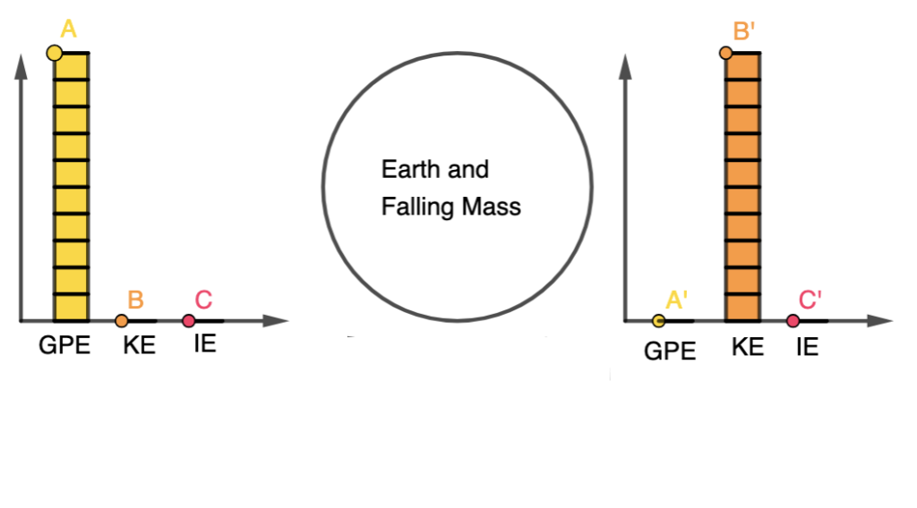
Here’s a breakdown of how LOL diagrams are used, using an example of a falling mass:
System Definition (O):
Choose what is part of the energy system (objects whose energies are being tracked) and what isn’t.
For example, in the case of a falling mass, the mass itself and the Earth are part of the energy system.
Initial State (L):
Represent the initial energy configuration of the system.
Identify the types of energy present in the system at the beginning. In this example, we begin with some gravitational potential energy.
Transition:
Show how energy changes as the system evolves. In the falling mass example, the gravitational potential energy decreases, and kinetic energy increases.
Final State (L):
Represent the energy distribution in the system at the end of the process.
In the falling mass example, at the point just before it hits the ground, kinetic energy is maximized, and gravitational potential energy is minimized.
LOL diagrams illustrate that energy within the system is conserved, meaning the total energy in the system remains constant.
External work (work done by forces outside the defined system) may impact the system’s energy, but internal work (work done within the defined system) does not change the total energy of the system.
The mathematical representation of the above problem will then simply be:
GPE = KE
This problem seems a bit trivial. Since LOL diagrams are a visual tool to help students and scientists analyze energy transformations and conservation, they can be used for making it easier to set up and solve conservation of energy equations in problems of greater complexity.
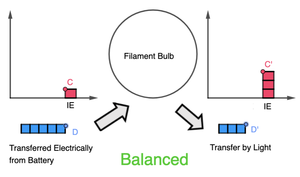
LOL Diagram of an Electrical Circuit
It is also important to note that the choice of the object (or system) of interest will result in different LOL diagrams for the same phenomenon.
For example, consider a filament bulb in a circuit with a battery. The system at room temperature also has some energy in the internal store (or internal energy, which consists of the kinetic and potential energies of the particles in the system).
When considering the filament as the object of interest, when energy is transferred electrically from the battery, part of it is transferred by light from the bulb to the surroundings and another part is added to the internal store, as it heats up the filament light.
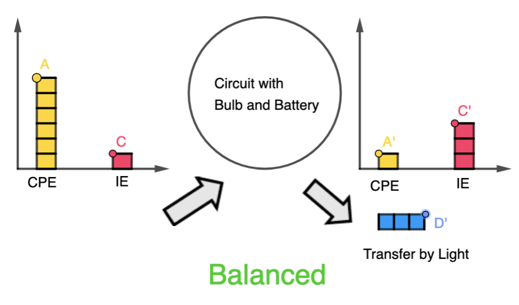
On the other hand, when considering the circuit as the whole, the chemical potential store of the battery is included in the initial energy state of the system. Hence, there is no additional energy transfer into the system but the energy transfer output is still the same.
How do I modify the GeoGebra applet to make my own LOL Diagram?
Here’s a video that demonstrates how the editing process is done, in a little more than one minute!